Overview

The system enables intuitive control through a Python-based application featuring a live 3D simulator that provides immediate visual feedback of arm positioning and reachability. Users can interact with the arm through direct manipulation in the simulation environment or program complex routines using generated G-code. The Arduino firmware performs real-time inverse kinematics calculations to convert 3D Cartesian coordinates into precise joint movements, while maintaining safety through software-enforced joint limits and hardware end stop monitoring.

Key achievements include developing a robust mathematical model for 3D positioning, creating a fluid user experience with real-time simulation, and implementing a reliable communication protocol that ensures smooth motion execution without serial communication bottlenecks.

Complete Demonstration

Here is a demonstration of the robot arm executing a programmed routine from generated G-code:

Programmed Motion Demo

Direct Control Mode

Real-time manipulation of the robot arm with live 3D simulation:

Direct Control Interface

Control Buttons:

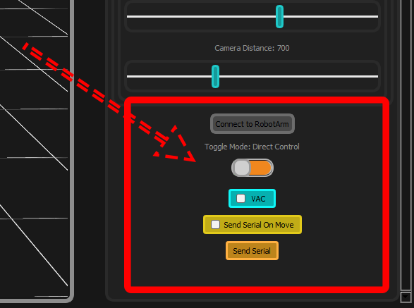
• Send on Move : Checkbox for real-time position updates to hardware during manipulation
• Send Serial Button : Manual command to send current position to the robot arm
• Vacuum Toggle : Direct control of end effector suction system

Orientation Controls:

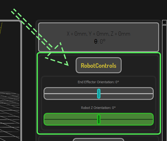
• Z Orientation Slider : Controls the angle of the kinematics plane
• End Effector Rotation : Adjusts the rotational position of the suction cup
• Live Synchronization : Real-time feedback between software and hardware

Intuitive Interaction System

The interface provides multiple control methods:

Click & Drag Positioning:

3D Orientation Control:

End Effector Rotation:

Interactive Camera System

The 3D simulator features comprehensive camera controls for optimal visualization:

Camera Control Interface:

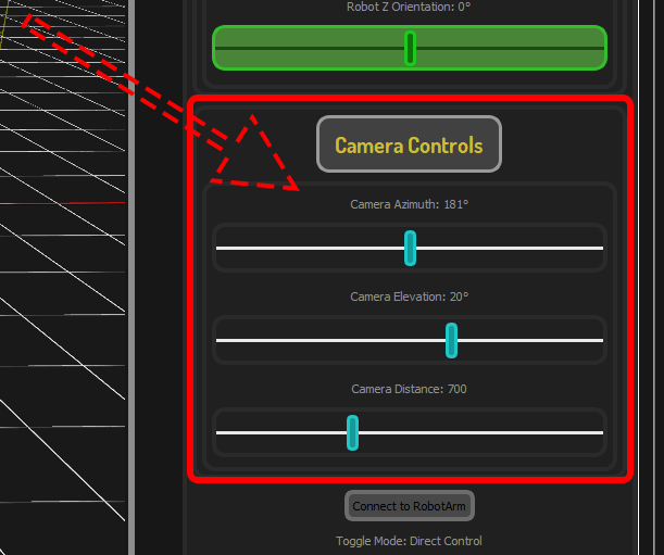
Azimuth Rotation (360° horizontal viewing):

Elevation Control (-90° to +90° vertical angle):

Zoom Distance (10mm to 2000mm range):

Direct Control Demo

G-Code Programming Modes

Two approaches for creating robot routines:

Interaction Buttons

The buttons by which we can interact with the g-code generator/editor are:

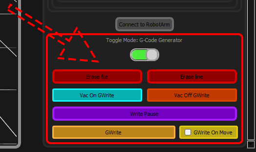
• Erase file : Wipes the temporary g-code file that holds the currently loaded g-code
• Erase line : Removes the last G-Code line from the file
• VAC On GWrite : Adds G-Code to activate the suction system
• VAC Off GWrite : Adds G-Code to deactivate the suction system
• Write Pause : Opens a dialog to insert dwell time in milliseconds
• GWrite : Writes the current simulated arm position to the g-code file
• GWrite On Move : Toggle that automatically records position changes (capped at 1 line per 100ms)

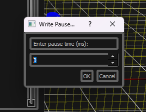
Pause/Dwell Dialog System

Features:

• Time Input : Numerical entry for dwell duration in milliseconds
• G-code Generation : Automatic creation of G04 dwell commands
• Seamless Integration : Direct insertion into current G-code program

G-Code Editor Controls

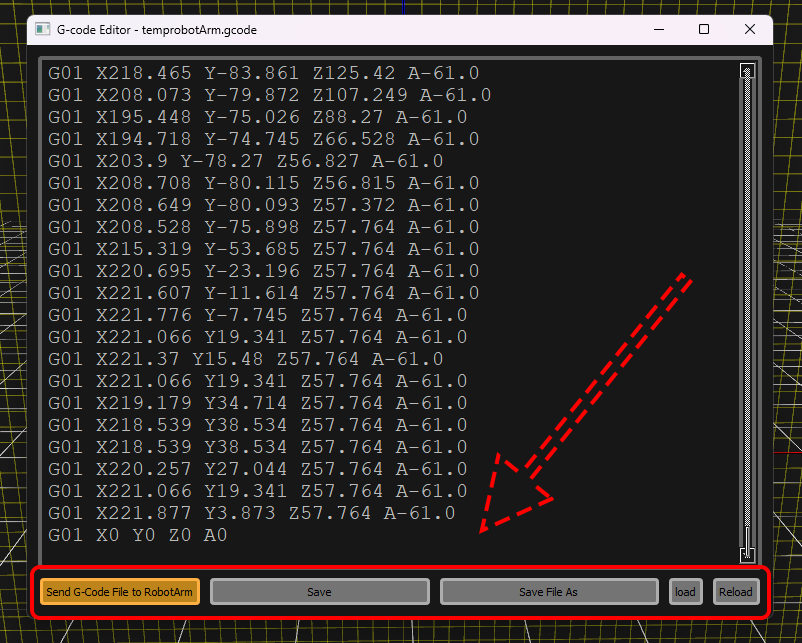
Editor Buttons:

• Send G-Code File to Robot Arm : Initiates transfer in 16-line batches with progress tracking
• Save : Saves current state of temporary file after direct edits
• Save File As : Exports temporary file for future loading
• Load : Imports external G-Code file into live editor
• Reload : Discards unsaved changes and reloads temporary file

G-Code Transfer Progress

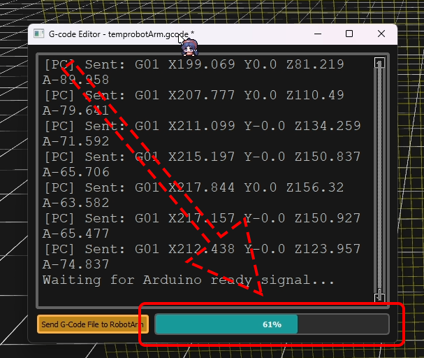
Progress Monitoring:

• Visual Indicator : Real-time progress bar showing transfer completion
• Status Feedback : Detailed messages on transfer state
• Batch Processing : 16-line batches with handshake protocol

Manual Write Mode - Precise point-to-point programming:

Write On Move Mode - Dynamic motion capture for fluid paths:

Tech Stack

Hardware

• Robotic Arm: 4-DOF SCARA-like arm with rotational base
• Microcontroller: Arduino Mega 2560
• Motion System:
• 4x NEMA 17 stepper motors with A4988 drivers
• Custom gear ratios for each joint (16:1 microstepping)
• End Effector: Vacuum suction system with PWM control
• Sensing: 4x mechanical endstops for homing and safety
• Cooling: Active cooling system for motor drivers

Firmware (C++/Arduino)

• Core Framework : Arduino IDE with custom C++ libraries
• Motor Control :
  • AccelStepper library for individual motor control
  • MultiStepper for coordinated motion across all axes
• External Libraries
  • Array : Open-source library for fixed-size array management
• Custom Libraries :
  • 4AxisRobotArm : Core kinematics and motor management
• Key Features :
  • Real-time inverse kinematics computation
  • Double-buffered G-code execution
  • Software-enforced joint limits
  • Safety monitoring with automatic homing

Software (Python)

• GUI Framework: PyQt5 with Qt3D for hardware-accelerated graphics

• 3D Visualization:

  • PyOpenGL integration via Qt3D
  • Real-time robotic arm simulation
  • Interactive manipulation plane

• Serial Communication: PySerial with multithreaded implementation

• Additional Libraries:

  • Standard math library for trigonometric calculations
  • Time library for rate limiting and timing control
  • SYS library for application management

Communication Protocol

• Physical Layer: Serial USB at 115,200 baud
• Data Format: Custom G-code dialect with batch processing
• Flow Control: Double-buffered system with handshake protocol

Mathematical Foundation

• Kinematics: Trigonometric inverse kinematics for 3D positioning
• Coordinate Systems: Multiple space transformations (world, plane, joint)
• 3D Math: Quaternion-based rotations and transformations

Hardware Deep Dive

Mechanical Assembly & Joint Configuration

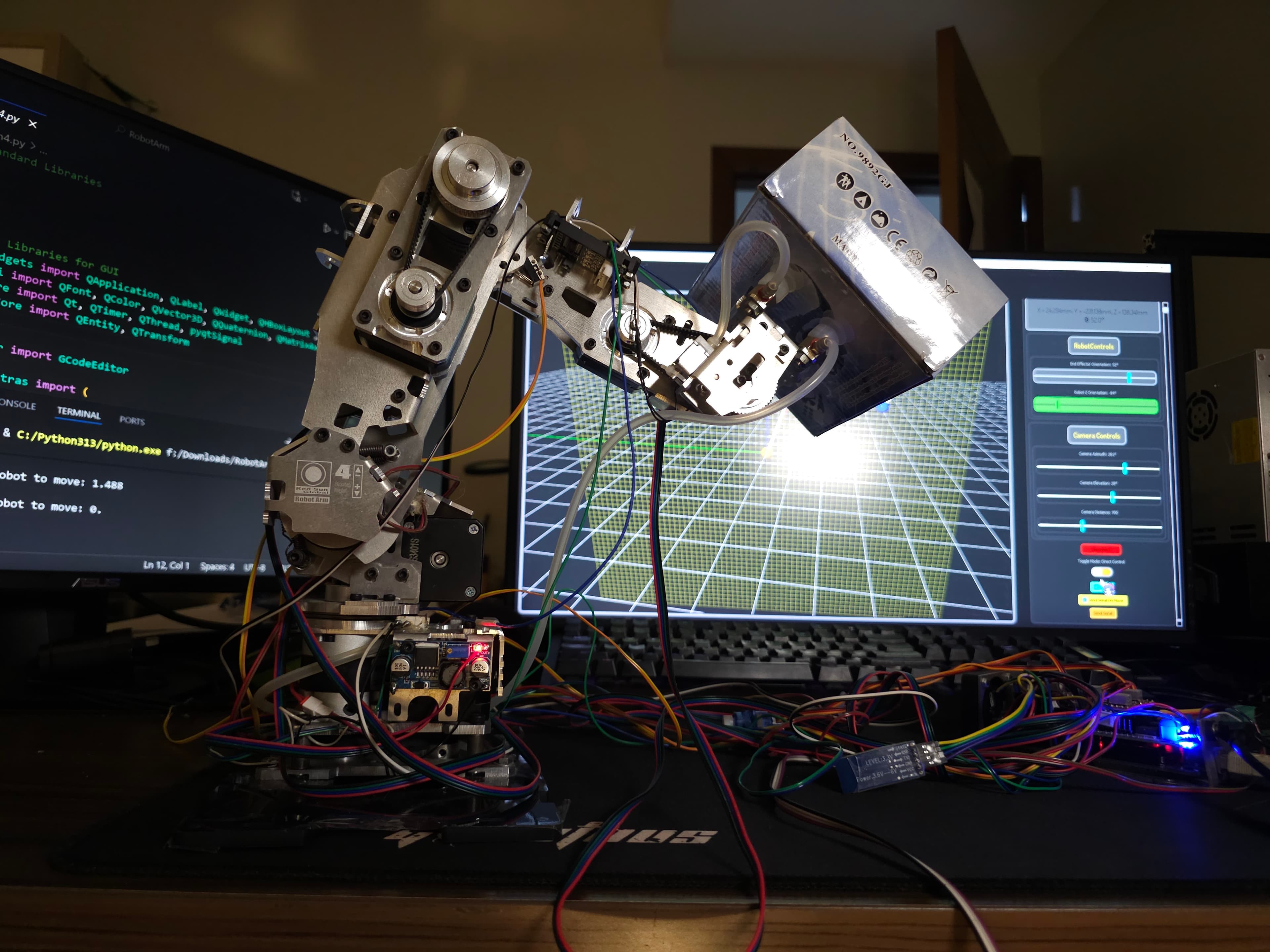
The robot arm features a 4-DOF (Degree of Freedom) SCARA-like design with a rotational base, providing comprehensive 3D positioning capabilities:

Joint Architecture

• Joint 1 (Base): 258° rotational base providing horizontal movement (-129° to +129°)
• Joint 2 (Shoulder): Primary lifting joint with 70° range (25° to 95°)
• Joint 3 (Elbow): Secondary arm joint with 135.5° range (52.5° to 188°)
• Joint 4 (Wrist): End effector orientation with 169.5° range (85° to 254.5°)

# =============================================
# ROBOT ARM LENGTHS (mm)
# =============================================

L1 = 159  # Base to elbow length
L2 = 155  # Elbow to wrist length
L3 = 58   # Wrist to end-effector length

# =============================================
# JOINT LIMITS
# =============================================

THETA1LIMIT = (-129, 129)
THETA2LIMIT = (25, 95)
THETA3LIMIT = (53, 180)
THETA4LIMIT = (95, 254)

The Degrees-Per-Step Calibration Challenge

The Problem: Unknown Gear Ratios

During assembly, I encountered a significant challenge: the gear ratios for each joint were undocumented and inaccessible without disassembling the arm. Traditional calculation methods were impossible, requiring an innovative empirical approach.

The Solution: Photogrammetric Approximation with Modern Tools

I developed a practical calibration method combining smartphone technology with CAD analysis:

Precision Setup Configuration:

• Smartphone Integration: Used phone's internal gyroscope and accelerometer to achieve near-perfect 90° alignment to the arm's movement plane
• Camera Positioning: Phone mounted on stable tripod, with sensor data ensuring orthogonal positioning

Iterative Measurement Process:

1. Set Movement : Commanded the arm to move fixed step increments
2. Visual Documentation : Captured before/after photos with smartphone
3. CAD Analysis : Imported images into AutoCAD for angular measurement
4. Trial and Refinement : Tested different step counts and repeated measurements
5. Practical Validation : Verified calibration accuracy by visually comparing end effector positioning between simulation predictions and physical arm behavior.

The Unexpected Results: When "Correct" Math Gives Wrong Answers

The approximation process revealed a surprising engineering paradox:

Initial Success with Practical Approach:

• Practical Approximations : My empirical measurements produced stable performance with minimal end-effector orientation drift
• System Behavior : The arm maintained consistent tool orientation and predictable motion paths

The Disappointing Realization:

When I later obtained the actual gear ratios from the manufacturer and implemented them:

• Calculated Values : Produced significantly worse performance with noticeable end-effector orientation drift
• Performance Regression : The mathematically "correct" values degraded system accuracy

The Critical Insight: Sometimes Physical Approximation Trumps Expected Specifications

This revealed that my photogrammatic method had unknowingly compensated for potential inaccuracies in manufacturer specifications and real-world assembly variations. The photogrammetric approach captured the true behavior of the complete mechanical system, accounting for factors that theoretical calculations missed.

Implementation

The empirically measured values were integrated into the firmware, producing:

• Stable end effector orientation across the entire workspace
• Predictable tool behavior during complex motions
• Reliable performance for pick-and-place operations

  ///Defining the constructers of the stepper Struct
  //Constructor to Handle auto calculation of DegPerStep
  stepper::stepper(byte stepPin, byte dirPin, byte enPin, byte endSwitchPin, double LowRange, double HighRange, long MotorStepsRange){

    this->stepPin = stepPin;
    this->dirPin = dirPin;
    this->enPin = enPin;
    this->endSwitchPin = endSwitchPin;
    this->LowRange = LowRange;
    this->HighRange = HighRange;
    this->MotorStepsRange = MotorStepsRange;
    DegPerStep = fabs(HighRange - LowRange) / MotorStepsRange;

    }

Key Engineering Lesson Learned

This experience revealed that physical measurement can outperform theoretical calculations when working with complex mechanical systems. The empirical approach succeeded because it captured:

• Real-world assembly variations and mechanical tolerances
• Potential inaccuracies in manufacturer specifications
• Compound effects of backlash and system compliance
• The true emergent behavior of the complete mechanical system

While mathematical models provide an essential foundation, physical validation remains the ultimate test of system performance, especially when dealing with assemblies where not all parameters can be perfectly known or verified.

Mathematical Foundation: Inverse Kinematics Implementation

Overview

The core of the robot arm control system lies in the inverse kinematics algorithm that converts 3D Cartesian coordinates into precise joint angles. Unlike many robotic systems that use complex matrix transformations, I implemented a trigonometric approach that's both computationally efficient and intuitively understandable.

The Inverse Kinematics Algorithm

Core Function Structure

  ///@brief Converts X Y Z, and End Effector Angle into Robot Arm Angles 
  RobotArm::RobotAngles RobotArm::InverseKinematics3D(float x, float y, float z, float Orio){
    //Converts Our angle into radians
        double OrioRad = radians(Orio);

      /*Since this is 3D by virtue of Base Arm rotation We can convert this into 
        2D plane inverse kinematics, after finding the base roation */

        double theta0 = atan2(y,x); // Calculating base angle

      //Shifting to 2D Plane Kinematics
        
        double l = sqrt(square(x) + square(y)); //Calculating the X Coordinate in the New plane
                                                // Z Axis becomes the new Y Axis

        double Xw = l - (ArmLength3 * cos(OrioRad)); // Calulating the X Coordinate of the 3rd Joint
        double Yw = z - (ArmLength3 * sin(OrioRad)); // Calculating the Y Coordinate of the 3rd Joint

        //Finding Joint2 Angle With some trig
          double r = sqrt( square(Xw) + square(Yw));
          double theta2 = acos(constrain((square(ArmLength1) + square(ArmLength2) - square(r))/(2.0 * ArmLength1 * ArmLength2), -1, 1));

        //Finding Joint1 Angle With some trig

          double thetaA = atan2(Yw,Xw);
          double thetaB = acos(constrain((square(r) + square(ArmLength1) - square(ArmLength2))/(2.0 * ArmLength1 * r), -1, +1));

          double theta1 = thetaA + thetaB; // Adding both Angles to compute Angle of th first joint
        
        //Finding third joint Angle using end effector Angle

          double theta3 = OrioRad - theta1 - theta2;

        //Converting Radians to Degrees

          double theta0deg = degrees(theta0);
          double theta1deg = degrees(theta1);
          double theta2deg = degrees(theta2);
          double theta3deg = degrees(theta3);
        //Making sure theta3 is positive;
          if(theta3deg < 0){
            theta3deg += 360; //Adding 360 degrees to negative theta3 angle to turn positive
          }
        
        //Returning theta values
        //RobotAngles Angles;
        Angles.theta0 = theta0deg;
        Angles.theta1 = theta1deg;
        Angles.theta2 = theta2deg;
        Angles.theta3 = theta3deg;

        return Angles;
      }
  

Step-by-Step Mathematical Derivation

1. Base Rotation (θ₀) - Handling 3D Space

The first step converts the 3D problem into a 2D plane problem by calculating the base rotation:

        double theta0 = atan2(y,x); // Calculating base angle

      //Shifting to 2D Plane Kinematics
        
        double l = sqrt(square(x) + square(y)); //Calculating the X Coordinate in the New plane
                                                // Z Axis becomes the new Y Axis

This effectively reduces the problem to a 2D arm in the calculated plane, with l becoming the new X coordinate and Z becoming the new Y coordinate.

2. Wrist Position Calculation

To solve for the joint angles, we first find the wrist position by accounting for the end effector length:

        double Xw = l - (ArmLength3 * cos(OrioRad)); // Calulating the X Coordinate of the 3rd Joint
        double Yw = z - (ArmLength3 * sin(OrioRad)); // Calculating the Y Coordinate of the 3rd Joint

3. Joint Angle Calculation Using Law of Cosines

The core of the algorithm uses the law of cosines to find the joint angles:

For θ₂ (Elbow Joint):

        //Finding Joint2 Angle With some trig
          double r = sqrt( square(Xw) + square(Yw));
          double theta2 = acos(constrain((square(ArmLength1) + square(ArmLength2) - square(r))/(2.0 * ArmLength1 * ArmLength2), -1, 1));

For θ₁ (Shoulder Joint):

          double thetaA = atan2(Yw,Xw);
          double thetaB = acos(constrain((square(r) + square(ArmLength1) - square(ArmLength2))/(2.0 * ArmLength1 * r), -1, +1));

          double theta1 = thetaA + thetaB; // Adding both Angles to compute Angle of th first joint

4. Wrist Angle Calculation

The wrist angle completes the kinematic chain:

          double theta3 = OrioRad - theta1 - theta2;

Coordinate System Transformations

The system manages multiple coordinate spaces:

1. World Coordinates (X, Y, Z): Global 3D position
2. Plane Coordinates (l, z): 2D working plane after base rotation
3. Joint Space (θ₀, θ₁, θ₂, θ₃): Motor angles
4. Step Counts : Actual stepper motor positions

Practical Implementation Details

Constraint Enforcement

The algorithm includes safety constraints to prevent mathematical errors by preventing arc cosine domain errors by constraining input to [-1, 1]:

          double theta2 = acos(constrain((square(ArmLength1) + square(ArmLength2) - square(r))/(2.0 * ArmLength1 * ArmLength2), -1, 1));

        //Finding Joint1 Angle With some trig

          double thetaA = atan2(Yw,Xw);
          double thetaB = acos(constrain((square(r) + square(ArmLength1) - square(ArmLength2))/(2.0 * ArmLength1 * r), -1, +1));

Multi-Layer Joint Limit Validation

The system implements a triple-layer safety approach to joint limit enforcement, providing redundant protection at every stage of the motion pipeline:

Layer 1: Simulation-Level Constraints (Python)

In the 3D simulation software, joint limits are enforced during inverse kinematics calculation to prevent invalid positioning in the virtual environment:

# =============================================
# JOINT LIMITS
# =============================================

THETA1LIMIT = (-129, 129)
THETA2LIMIT = (25, 95)
THETA3LIMIT = (53, 180)
THETA4LIMIT = (95, 254)

def clamp_angle(angle: float, limits: tuple[float, float]) -> float:
    """
    Clamps the angle between the specified limits.

    :param angle: float — the input angle
    :param limits: tuple or list (min_angle, max_angle)
    :return: float — clamped angle
    """
    min_angle, max_angle = limits
    return max(min(angle, max_angle), min_angle)

Layer 2: Firmware Angle Constraints (C++)

After calculating joint angles in the inverse kinematics, the firmware constrains the output to physical limits before motion execution:

  void RobotArm::MoveRobotArmJoints(double ZOrio, double Joint1Angle, double Joint2Angle, double Joint3Angle){

          ZOrio = constrain(ZOrio, -(stepper1.HighRange - stepper1.LowRange) / 2, (stepper1.HighRange - stepper1.LowRange) / 2); //Constraining to angular Range

          Joint1Angle = constrain(Joint1Angle, stepper2.LowRange, stepper2.HighRange);

          Joint2Angle = constrain(Joint2Angle, stepper3.LowRange, stepper3.HighRange);

           Joint3Angle = constrain(Joint3Angle, stepper4.LowRange, stepper4.HighRange);

Layer 3: Step-Level Range Checking (C++)

After converting angles to step counts, the system performs a final validation to ensure steps remain within safe mechanical ranges:

        // Constrain steps if MaxStepRange is available
          if(stepper2.MotorStepsRange > 0){
            Joint1Steps = constrain(Joint1Steps, 0, stepper2.MotorStepsRange);
          }

          if(stepper3.MotorStepsRange > 0){
            Joint2Steps = constrain(Joint2Steps, 0, stepper3.MotorStepsRange);
          }

        // Constrain steps if MaxStepRange is available
          if(stepper4.MotorStepsRange > 0){
            Joint3Steps = constrain(Joint3Steps, 0, stepper4.MotorStepsRange);
          }

Safety Architecture Benefits

This triple-layer approach provides:

1. Preventive Safety : Simulation prevents users from even attempting invalid positions
2. Corrective Safety : Firmware automatically corrects any miscalculated angles
3. Absolute Safety : Step-level constraints provide hardware-level protection
4. Redundant Protection : Each layer can catch errors missed by previous layers

Implementation in Motion Pipeline

The complete safety chain works as:

3D Position → Inverse Kinematics → Layer 1 (Python Constraints)
    → Layer 2 (Angle Constraints) → Step Conversion
    → Layer 3 (Step Constraints) → Physical Movement

This comprehensive approach ensures that even if one validation layer fails, subsequent layers will prevent the arm from attempting physically impossible or dangerous movements, providing robust protection for both the hardware and surrounding environment.

The system demonstrates professional-grade safety engineering, where multiple independent validation mechanisms work together to create a fault-tolerant motion control system.

Numerical Stability

The implementation handles edge cases and numerical precision:

• Uses atan2() instead of atan() for correct quadrant handling
• Applies constraints to prevent acos() domain errors
• Maintains angle consistency with degree/radian conversions

Integration with Motion Control

The inverse kinematics function feeds directly into the joint control system:

  void RobotArm::MoveRobotArmToPosition(double x, double y, double z, double Orio){
    RobotAngles Angles = InverseKinematics3D(x, y, z, Orio); // Calculates Robot Arm Angles
    MoveRobotArmJoints(Angles.theta0, Angles.theta1, Angles.theta2, Angles.theta3); //Moves Robot Arm Angles to that position
    }

Key Mathematical Insights

1. Trigonometric Efficiency : The law of cosines approach is computationally lighter than matrix transformations, making it ideal for real-time control on limited hardware.
2. Geometric Intuition : Each mathematical step corresponds to a clear geometric relationship, making the algorithm debuggable and understandable.
3. Constraint Propagation : Joint limits and physical constraints are naturally incorporated into the mathematical model.
4. Coordinate System Management : The systematic transformation between coordinate spaces ensures consistent positioning across the entire workspace.

This mathematical foundation demonstrates how classical trigonometry, when carefully applied, can solve complex 3D positioning problems with elegance and computational efficiency.

Software Architecture: PyQt5 3D Simulation & Control System

Overview

The robot arm control software is built around a sophisticated PyQt5 application that provides real-time 3D visualization, intuitive control interfaces, and seamless hardware integration. The architecture follows a modular design pattern where each subsystem handles specific responsibilities while maintaining clean interfaces.

Core Architecture

Main Application Controller

The Robot3DSimulator class serves as the central coordinator, managing:

• 3D Visualization Engine using Qt3D for hardware-accelerated rendering
• Dynamic UI System with mode-based control panels
• Serial Communication Manager with multithreaded operation
• Real-time Kinematics Calculator for position updates
• G-code Generation Pipeline for program creation

Multi-Layer UI System

The interface employs a sophisticated layout system that allocates approximately 75% of screen space to the 3D visualization and 25% to the control panels. This balance ensures the simulation remains the primary focus while providing comprehensive control access. The control panel itself uses a scrollable area with stacked widgets to elegantly switch between operational modes, maintaining a compact yet fully-featured interface.

Key Subsystems

3D Visualization Engine

The Qt3D-based rendering system creates an immersive simulation environment featuring a hierarchical scene graph for efficient transformations, real-time camera control using spherical coordinates, an interactive manipulation plane with object pickers for direct control, and a visual feedback system with color-coded reachability indicators that provide immediate user feedback.

Dual-Mode Operating System

The software supports two primary operational modes with distinct characteristics. Direct Control Mode enables real-time serial communication with physical hardware, providing immediate visual feedback in the 3D simulation and supporting interactive positioning. G-code Generator Mode focuses on offline path planning and animation capture, offering two writing methods and an integrated editor with live preview capabilities.

Real-time Kinematics Pipeline

The inverse kinematics system operates continuously, converting 3D positions to 2D plane coordinates, calculating inverse kinematics solutions, and updating joint transforms in the 3D scene. This pipeline ensures the simulation stays perfectly synchronized with both mathematical calculations and user inputs.

Advanced Features

Intelligent Event Handling

The system implements sophisticated event management including rate-limited updates to prevent UI flooding during rapid movements, drag-and-drop interaction with visual feedback spheres, and multithreaded communication to prevent blocking during serial operations.

Comprehensive Styling System

A centralized styling architecture provides consistent theming across all interface elements, with over twenty distinct style definitions managing colors, borders, spacing, and visual effects to create a professional and cohesive user experience.

Camera Control System

Flexible viewing options are provided through three independent sliders controlling azimuth for 360° horizontal rotation, elevation for -90° to +90° vertical angle adjustment, and distance for 10mm to 2000mm zoom range, giving users complete control over their viewing perspective.

Performance Optimization

The architecture employs several optimization strategies including non-blocking operations using QThread for serial communication, efficient 3D rendering through Qt3D's hardware acceleration, smart update scheduling to minimize computational overhead, and memory-conscious object management with proper parent-child relationships.

Integration Patterns

The software demonstrates several key integration patterns: the Observer Pattern allows UI components to react to state changes automatically, the Strategy Pattern enables interchangeable operational modes, the Factory Pattern supports dynamic creation of UI components based on mode, and the Bridge Pattern maintains clear separation between simulation and hardware layers.

This architecture creates a robust, maintainable, and extensible foundation for robotic control applications, balancing real-time performance with rich user experience through careful subsystem design and efficient inter-component communication.

Firmware Design: Arduino Motion Control System

Overview

The robot arm firmware represents a complete ground-up redesign of the original control system, built around a custom 4AxisRobotArm library that provides sophisticated motion control, inverse kinematics computation, and G-code interpretation. The firmware operates as a real-time control system that balances computational demands with precise timing requirements.

Core Architecture

Main Control Loop

The firmware follows a classic embedded systems architecture with a super-loop design. The main loop continuously processes incoming G-code commands while managing stepper motor movements, ensuring smooth coordinated motion across all four axes. The system maintains real-time responsiveness by separating command processing from motion execution.

Double-Buffered Command System

A sophisticated double-buffering system prevents serial communication from blocking motion execution:

• Primary Buffer : Receives and parses incoming G-code lines from serial
• Active Buffer : Supplies pre-parsed commands for execution
• Seamless Transition : Automatic buffer swapping when active buffer empties

This architecture allows the arm to execute complex motions while simultaneously receiving new commands, eliminating motion stuttering during file transfers.

Custom 4AxisRobotArm Library

Stepper Management System

The library abstracts low-level motor control through a structured approach:

  }
  ///Defining the constructers of the stepper Struct
  //Constructor to Handle auto calculation of DegPerStep
  stepper::stepper(byte stepPin, byte dirPin, byte enPin, byte endSwitchPin, double LowRange, double HighRange, long MotorStepsRange){

    this->stepPin = stepPin;
    this->dirPin = dirPin;
    this->enPin = enPin;
    this->endSwitchPin = endSwitchPin;
    this->LowRange = LowRange;
    this->HighRange = HighRange;
    this->MotorStepsRange = MotorStepsRange;
    DegPerStep = fabs(HighRange - LowRange) / MotorStepsRange;

    }

  //Constructor to Handle manual input of DegPerStep
  stepper::stepper(byte stepPin, byte dirPin, byte enPin, byte endSwitchPin, double LowRange, double HighRange, double DegPerStep ,long MotorStepsRange){

    this->stepPin = stepPin;
    this->dirPin = dirPin;
    this->enPin = enPin;
    this->endSwitchPin = endSwitchPin;
    this->LowRange = LowRange;

Each stepper instance encapsulates complete motor configuration, including pin assignments, angular ranges, and step-to-degree conversions. The library supports both automatic calculation from empirical parameters and manual specification for mechanical ratios.

Inverse Kinematics Engine

The firmware implements the same trigonometric inverse kinematics algorithm as the Python software, ensuring mathematical consistency between simulation and physical execution. The C++ implementation optimizes for computational efficiency while maintaining floating-point precision for accurate positioning.

Motion Planning & Coordination

The MultiStepper library coordinates simultaneous movement across all axes, ensuring joints arrive at their destinations synchronously. The system calculates appropriate speeds for each motor based on their individual travel distances, preventing overshoot and ensuring smooth, coordinated motion.

G-code Processing Pipeline

Custom Parser Implementation

The firmware implements a robust G-code parser that handles the custom command dialect:

/// @brief Struct to store Gcodeline info
struct Gcode{

  char mode[4];
  double x;
  double y;
  double z;
  double A;
  double B;
  double C;
  double f;
  double P;

  void print(){
    Serial.print("X: ");
    Serial.print(x);
    Serial.print(", Y: ");
    Serial.print(y);
    Serial.print(", Z: ");
    Serial.print(z);
    Serial.print(", A: ");
    Serial.print(A);
    Serial.print(", B: ");
    Serial.print(B);
    Serial.print(", C: ");
    Serial.print(C);
    Serial.print(", F: ");
    Serial.print(f);
    Serial.print("\n");
  }
  Gcode(char mode[4], double x, double y, double z, double A, double B, double C, double f, double P)
  : x(x), y(y), z(z), A(A), B(B), C(C), f(f), P(P){
    strncpy(this->mode,mode,3);
    this->mode[3] = '\0';
  }

  Gcode(){}
  


};

The parser extracts parameters using string scanning techniques, supports comment stripping, and handles missing parameters through state persistence across commands.

Command Execution Logic

The system processes multiple command types:

• G01 (Linear Move) : Position moves with coordinated motion
• M03/M05 (Vacuum Control) : End effector activation commands
• G04 (Dwell) : Precision timing pauses
• State Persistence : Parameters carry forward until explicitly changed

Safety Systems

Multi-Layer Protection

The firmware implements comprehensive safety measures:

• Software Endstops : Constrain joint angles to mechanical limits
• Hardware Endstops : Physical limit switches for emergency stops
• Step Range Validation : Final verification before movement execution
• Automatic Homing : Recovery procedure after limit triggers

Emergency Response

When endstops activate, the firmware immediately disables affected motors and initiates homing sequences. The system provides detailed serial feedback during recovery operations, allowing the host software to monitor and respond to fault conditions.

Real-time Performance

Timing-Critical Operations

The firmware maintains precise timing through:

• Non-blocking Stepper Control : AccelStepper library for interrupt-driven pulse generation
• Efficient Kinematics : Optimized floating-point calculations
• Predictable Loop Timing : Consistent execution time per cycle
• Buffer Management : Prevention of serial overflow conditions

Memory Management

Despite the Arduino Mega's limited RAM, the system efficiently manages memory through:

• Fixed-size Buffers : Prevents heap fragmentation
• Stack-based Allocation : Minimizes dynamic memory usage
• Structure Packing : Optimized data structure layout

Communication Protocol

Serial Interface Design

The firmware implements a robust serial protocol:

• 115,200 Baud Rate : Balance between speed and reliability
• Line-based Protocol : Simple parsing with newline delimiters
• Flow Control : Ready signals for batch processing
• Error Reporting : Status feedback to serial monitor

G-code Batch Processing

Commands are processed in configurable batches (default 16 lines) with handshake protocol:

1. Host sends batch of commands
2. Firmware executes while parsing next batch
3. Firmware requests next batch when ready
4. Continuous pipeline maintains smooth motion

Integration with Control Software

The firmware maintains perfect synchronization with the Python control software through shared mathematical models and consistent coordinate systems. This ensures that simulated motions translate accurately to physical movements, creating a seamless development and operation experience.

The firmware design demonstrates how careful architecture can overcome hardware limitations to deliver professional-grade motion control, providing a robust foundation for complex robotic applications while maintaining safety and reliability.

Communication Protocol: Custom G-code & Serial Handshaking

Overview

The communication system between the Python control software and Arduino firmware implements a sophisticated protocol that ensures reliable data transfer, efficient motion execution, and robust error handling. The design balances human-readability with machine efficiency.

Custom G-code Dialect

Command Structure

The system uses a customized G-code implementation that extends standard syntax:

G01 X10.5 Y20.3 Z5.0 A-45.0 F100.0  ; Linear move with feed rate
M03                                  ; Vacuum on
M05                                  ; Vacuum off  
G04 P1000                            ; Dwell for 1000ms

Parameter Persistence

The protocol implements stateful parameter handling:

• Unspecified parameters maintain previous values
• Allows compact command sequences
• Reduces serial bandwidth requirements

Serial Communication Architecture

Physical Layer

• Baud Rate : 115,200 for optimal speed/reliability balance
• Data Format : 8N1 (8 data bits, no parity, 1 stop bit)
• Flow Control : Software-based handshaking

Message Protocol

Double-Buffered Processing System

Buffer Architecture

The firmware implements a sophisticated double-buffer system:

// Intialising Gcode Buffer
  Array<Gcode, 16> gcodeBuffer;
  Array<Gcode, 16> ActivegcodeBuffer;

Flow Control Mechanism

1. Host sends 16-line batches to receiving buffer
2. Firmware processes from active buffer while receiving
3. Buffer swap occurs when active buffer empties
4. Ready signal sent when buffers need refilling

Batch Processing Protocol

Transmission Sequence

HOST: [Batch of 16 G-code lines]
ARDUINO: Executes commands while parsing
ARDUINO: "Gcode Buffer Is Empty" (ready for more)
HOST: [Next batch of 16 lines]

Advantages

• Continuous Motion : No pauses between command batches
• Memory Efficiency : Fixed buffer sizes prevent overflow
• Error Resilience : Small batches minimize data loss

G-code Parser Implementation

Robust Parsing Logic

The firmware parser handles:

• Comment Stripping : Removes ";" and trailing comments
• Case Insensitivity : Converts commands to uppercase
• Parameter Extraction : Flexible field detection
• Error Resilience : Graceful handling of malformed commands

Parameter Detection

  index = GcodeLine.indexOf('X'); //Find index of X
  // Find X if passed
  if (index != -1){
    //Find index of whiteSpace After X or end terminator
      int index2 = GcodeLine.indexOf(" ", index);
      if(index2 == -1){
        index2 = GcodeLine.length();
      }
   X = GcodeLine.substring(index + 1, index2).toDouble();
  }

Error Handling

• Serial Timeouts : Prevents blocking on incomplete data
• Buffer Full Detection : Flow control to prevent data loss
• Command Validation : Robust parsing of G-code parameters

Multithreaded Host Implementation

Python Communication Thread

The GCodeSenderThread class handles batch processing with real-time progress reporting, non-blocking serial communication, and automatic error handling while keeping the main UI responsive.

Features

• Progress Reporting : Real-time status updates to UI
• Non-blocking Operation : Main UI remains responsive during file transfers
• Automatic Recovery : Handles serial disconnects gracefully

Protocol Efficiency

Bandwidth Optimization

• State Persistence : Only changed parameters need transmission
• Batch Processing : Reduced protocol overhead through command grouping
• Compact Format : Minimal whitespace and efficient parameter encoding

Reliability Measures

• Line-based Protocol : Simple and robust parsing
• Flow Control : Prevents buffer overruns in both directions
• Timeout Handling : Recovers from communication interruptions

This communication protocol demonstrates how careful design can overcome the limitations of simple serial links, creating a robust, efficient, and maintainable system that supports both interactive control and complex automated operations.

Challenges & Lessons Learned

Technical Challenges

The 3D Interaction Struggle

The most significant technical challenge was implementing the 3D mouse interaction system. My initial attempt using OpenGL failed completely—I couldn't get the ray-plane intersection to work at all despite extensive effort. The documentation was confusing, and none of the methods I tried functioned reliably.

Faced with this fundamental roadblock, I made the difficult decision to completely abandon OpenGL and rebuild the entire 3D visualization system using PyQt3D. This rewrite proved to be the right choice, as PyQt3D provided a much more robust foundation.

However, even in PyQt3D, I encountered another hurdle. By default, the system would detect a "hit" if the mouse pointer intersected with an object's overall bounding box—a rough, invisible cage around the object. This meant clicking my orientation plane would register as a hit on the bounding box, and not the plane itself.

After extensive testing, I discovered a poorly documented setting that switched the system to precise, triangle-level intersection. This meant a hit was only registered if the mouse pointer directly intersected the actual visible surface of the object. Once enabled, this setting transformed the interaction from unreliable to perfectly accurate, finally providing the precise 3D mouse control the project required.

The Documentation Gap

A crucial breakthrough came when testing intersection behaviors revealed that PyQt3D had a poorly documented "precise intersection" setting. Once enabled, this setting transformed the interaction from unreliable to perfectly accurate. This experience highlighted how critical persistence and experimental testing can be when working with under-documented frameworks.

Development Time Surprises

The Python software development consumed significantly more time than expected. What began as a simple control interface evolved into a complex 3D simulation environment with real-time kinematics, camera controls, and dual operational modes. The iterative process of refining the user experience and ensuring robust performance accounted for the majority of the project timeline.

Architectural Insights

Code Organization Regrets

If starting over, I would implement a more modular architecture from the beginning. The current single-file Python implementation, while functional, would benefit from separation into discrete modules for 3D rendering, serial communication, inverse kinematics, and UI components. This would improve maintainability and testing efficiency.

Hardware Documentation Lesson

A critical lesson learned: always document gear and pulley ratios before assembling robotic systems. The extensive calibration process required to reverse-engineer these ratios after assembly represented significant avoidable work. Future projects will include thorough mechanical documentation during the build phase.

Performance Realities

Hardware Limitations

The Arduino Mega's computational limits necessitated compromises in motion coordination. Despite careful optimization, floating-point inaccuracies and processing speed constraints prevent perfectly synchronized motor stopping. This hardware-bound limitation represents the trade-off between cost and performance in embedded systems.

Communication Complexity

The G-code Transfer Challenge

Serial communication appeared straightforward in theory but revealed hidden complexities in practice. Implementing reliable G-code file transfer with proper flow control, error handling, and progress reporting required multiple iterations. The final double-buffered batch system emerged from overcoming these communication hurdles.

Mathematical Translation Headaches

Converting calculated joint angles into precise stepper motor steps proved unexpectedly challenging. The translation required careful consideration of gear ratios, step resolutions, and coordinate system transformations. What seemed like simple arithmetic revealed subtle complexities in real-world implementation.

The Unforeseen Simplicity

Inverse Kinematics Revelation

The trigonometric mathematics underlying inverse kinematics initially appeared daunting. However, the derivation process revealed an elegant simplicity - the same fundamental relationships that seemed complex in abstract became intuitive when applied to the physical robot arm. This experience demonstrated how hands-on implementation can transform perceived complexity into understandable systems.

Key Engineering Takeaways

1. Persistence Over Documentation : When documentation fails, systematic testing and experimentation can reveal solutions
2. Hardware First : Mechanical parameters should be documented during assembly, not reverse-engineered afterward
3. Expect the Unexpected : Simple-sounding tasks often contain hidden complexities
4. Embrace Rewrites : Sometimes starting fresh with a better framework is more efficient than fighting inadequate tools
5. Theory vs Practice : Mathematical concepts often simplify when applied to concrete problems

These challenges ultimately strengthened the final system, each obstacle overcome contributing to a more robust and reliable robotic control platform.

Conclusion & Future Work

Project Success Summary

This project successfully demonstrates a complete, ground-up redesign of a robotic arm control system that bridges the gap between intuitive software interfaces and precise physical execution. The integrated solution provides:

• Real-time 3D Simulation : A sophisticated PyQt5-based interface with interactive manipulation and visual feedback
• Accurate Inverse Kinematics : Robust mathematical models that reliably convert 3D coordinates to joint movements
• Dual Operational Modes : Flexible control through both direct manipulation and programmed G-code sequences
• Robust Communication : A reliable serial protocol that ensures smooth data transfer between software and hardware
• Practical Calibration : Empirical methods that overcome theoretical limitations for real-world accuracy

The system represents a significant achievement in mechatronics integration, combining sophisticated software architecture with embedded systems design to create a professional-grade robotic control platform.

Technical Achievements

Software Innovation

The PyQt5 3D simulation environment sets a new standard for accessible robotic programming, providing laboratory-grade visualization and control through consumer hardware. The dual-mode interface successfully balances immediate interactivity with programmable automation.

Mathematical Foundation

The trigonometric inverse kinematics implementation proves that classical mathematics, when carefully applied, can solve complex 3D positioning problems with both computational efficiency and intuitive understanding.

Hardware Integration

The custom 4AxisRobotArm library demonstrates how thoughtful firmware design can overcome hardware limitations to deliver precise, reliable motion control while maintaining comprehensive safety systems.

Future Enhancements

Immediate Improvements

• Expanded G-code Support : Support for circular interpolation (G02/G03) and more CNC-standard commands
• Multiple Tool Support : Configurable end-effector profiles for grippers, sensors, and other tools
• Motion Teaching : Support for easy programming via moving the robot head with your own hand

Medium-term Development

• Computer Vision Integration : Camera-based object recognition and automated pick-and-place routines
• Network Connectivity : Web interface and remote operation capabilities
• Advanced Simulation : Physics-based modeling for payload handling and dynamic effects

Possible Long-term Vision

• Multi-arm Coordination : Synchronized control of multiple robotic arms
• AI-assisted Programming : Machine learning for motion optimization and task learning
• Industrial Integration : Compatibility with standard industrial automation protocols
• Educational Platform : Curriculum materials and simplified interfaces for STEM education

Broader Implications

This project demonstrates that sophisticated robotic control systems are accessible to dedicated makers and students, not just large institutions. The integration of modern software frameworks with embedded systems creates new possibilities for:

• Research Platforms : Affordable, customizable systems for academic and industrial research
• Prototyping Tools : Rapid development and testing of automated systems
• Educational Resources : Hands-on learning experiences in robotics and mechatronics
• Small-scale Automation : Cost-effective solutions for small businesses and workshops

Final Reflection

The journey from theoretical concept to functional system reinforced fundamental engineering principles: the importance of accurate measurement, the value of persistent problem-solving, and the power of integrating multiple technical disciplines. Each challenge overcome—from 3D interaction mathematics to serial communication protocols—contributed to a deeper understanding of both the specific technologies and the general principles of system design.

This project stands as testament to what can be achieved through careful planning, iterative development, and willingness to tackle complex, multi-domain problems. It provides not just a functional robotic control system, but a foundation for future innovation in accessible, sophisticated automation technology.

Source Code

The complete source code for this project is available:

Arduino Firmware

• Robot Arm Controller (INO) - Main firmware
• 4-Axis Robot Arm Library (CPP) - Motor control implementation
• Robot Arm Library Header (H) - Library interface definitions

Python Application

• 3D Robot Arm Simulator (PY) - Main control software
• Live Code Editor Module (PY) - G-code editing interface